Week 15 (8/10/18 - 12/10/18)

Statistics By Sehra Sir

We had been having sessions with Sukhjit Sehra Sir on statistics since the past week. This week we learned about the following topics:

Probability and Probability Distributions

Probability theory developed from the study of games of chance like dice and cards.  A process like flipping a coin, rolling a die or drawing a card from a deck is called probability experiments.  An outcome is a specific result of a single trial of a probability experiment.

Probability Distributions

Probability theory is the foundation for statistical inference.  A probability distribution is a device for indicating the values that a random variable may have.  There are two categories of random variables.  These are discrete random variables and continuous random variables.

Discrete random variable
The probability distribution of a discrete random variable specifies all possible values of a discrete random variable along with their respective probabilities.

Examples can be

• Frequency distribution
• Probability distribution (relative frequency distribution)
• Cumulative frequency

Examples of discrete probability distributions are the binomial distribution and the Poisson distribution.

Binomial distribution

A binomial experiment is a probability experiment with the following properties.

1.  Each trial can have only two outcomes which can be considered success or failure.
2.  There must be a fixed number of trials.
3.  The outcomes of each trial must be independent of each other.
4.  The probability of success must remain the same in each trial.

The outcomes of a binomial experiment are called a binomial distribution.

Poisson distribution
The Poisson distribution is based on the Poisson process.

1.  The occurrences of the events are independent in an interval.
2.  An infinite number of occurrences of the event are possible in the interval.
3.  The probability of a single event in the interval is proportional to the length of the interval.
4.  In an infinitely small portion of the interval, the probability of more than one occurrence of the event is negligible.

Continuous probability distributions

A continuous variable can assume any value within a specified interval of values assumed by the variable.  In a general case, with a large number of class intervals, the frequency polygon begins to resemble a smooth curve.

A continuous probability distribution is a probability density function.  The area under the smooth curve is equal to 1 and the frequency of occurrence of values between any two points equals the total area under the curve between the two points and the x-axis.

The normal distribution
The normal distribution is the most important distribution in biostatistics.  It is frequently called the Gaussian distribution.  The two parameters of the normal distribution are the mean (m) and the standard deviation (s).  The graph has a familiar bell-shaped curve.

Deep Learning Homework

As we had completed 3 videos of Biksha Sir's Deep Learning videos, there was a homework assigned to us. It entailed two problems: the first problem was to identify MNIST dataset's digits using back propagation, the second problem was speech recognition.

We solved the first problem this week.

For part 1 of the homework, we were to write our own implementation of the backpropagation
algorithm for training our own neural network. We were required to do this assignment in the Python (Python version 3) programming language and not to use any audodiff toolboxes (TensorFlow, Keras, PyTorch, etc) - we were allowed to use only numpy like libraries (numpy, pandas, etc).

The goal of this assignment was to label images of 10 handwritten digits of “zero”, “one”,...,
“nine”. The images are 28 by 28 in size (MNIST dataset), which we will be represented as a vector x of dimension 784 by listing all the pixel values in raster scan order. The labels t are 0,1,2,...,9 corresponding to 10 classes as written in the image. There are 3000 training cases, containing 300 examples of each of 10 classes.

The idea is to take a large number of handwritten digits, known as training examples,

and then develop a system which can learn from those training examples. In other words, the neural network uses the examples to automatically infer rules for recognizing handwritten digits. Furthermore, by increasing the number of training examples, the network can learn more about handwriting, and so improve its accuracy.

To recognize individual digits we will use a three-layer neural network:

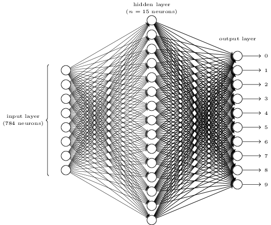
The input layer of the network contains neurons encoding the values of the input pixels. Our training data for the network will consist of many 2828 by 2828 pixel images of scanned handwritten digits, and so the input layer contains 784=28×28 neurons.  The input pixels are greyscaled, with a value of 0.0 representing white, a value of 1.0 representing black, and in between values representing gradually darkening shades of grey.

The second layer of the network is a hidden layer. We denote the number of neurons in this hidden layer by n and we'll experiment with different values for n. The example shown illustrates a small hidden layer, containing just n=15neurons.

The output layer of the network contains 10 neurons. If the first neuron fires, i.e., has an output ≈1, then that will indicate that the network thinks the digit is a 0. 

An idea called stochastic gradient descent can be used to speed up learning. The idea is to estimate the gradient ∇C by computing ∇Cx for a small sample of randomly chosen training inputs. By averaging over this small sample it turns out that we can quickly get a good estimate of the true gradient ∇C, and this helps speed up gradient descent, and thus learning.xzkcjnvlkmb,/xccvkn.cv.